Coronavirus Recovery Activity

Our task was to analyse coronavirus recovery data from India from January 2020 to March 2020 using RStudio.

The data came from here on Kaggle. Here's a sample of the data. (There are actually 270 rows.)

Sno	Date	State/UnionTerritory	ConfirmedIndianNational	ConfirmedForeignNational	Cured	Deaths
1	30-01-2020	Kerala	1	0	0	0
2	31-01-2020	Kerala	1	0	0	0
3	01-02-2020	Kerala	2	0	0	0
4	02-02-2020	Kerala	3	0	0	0
5	03-02-2020	Kerala	3	0	0	0

First I created a frequency table to count how many daily reports came from each state.

table(Covid19_India_Jan_20_Mar_20_$`State/UnionTerritory`)

Here are the first few results.

State/UnionTerritory	Freq
Andhra Pradesh	10
Chandigarh	1
Chattisgarh	1
Chhattisgarh	2
Delhi	20

The results show that the states weren't named consistently, for example "Chhattisgarh" was named "Chattisgarh" in one record. I browsed the other records and saw that Union territories were also not named consistently, for example, "Ladakh" was sometimes named "Union Territory of Ladakh".

I used this R code to tidy the data.

library(dplyr)

#rename any states named "Chattisgarh"
Covid19_India_Jan_20_Mar_20_$`State/UnionTerritory` <- which(Covid19_India_Jan_20_Mar_20_$`State/UnionTerritory` == "Chattisgarh") %>% 
  replace(Covid19_India_Jan_20_Mar_20_$`State/UnionTerritory`, ., "Chhattisgarh")

#get row numbers of states starting with "Union Territory of "
ut <- which(substr(Covid19_India_Jan_20_Mar_20_$`State/UnionTerritory`, 1, 19) == "Union Territory of ")

#remove "Union Territory of " from the start of any state names
Covid19_India_Jan_20_Mar_20_$`State/UnionTerritory`[ut] <-
  substr(Covid19_India_Jan_20_Mar_20_$`State/UnionTerritory`[ut], 20, nchar(Covid19_India_Jan_20_Mar_20_$`State/UnionTerritory`[ut]))

I created the frequency table again with the corrected data.

table(Covid19_India_Jan_20_Mar_20_$`State/UnionTerritory`)

Here are the first few results.

State/UnionTerritory	Freq
Andhra Pradesh	10
Chandigarh	1
Chhattisgarh	3
Delhi	20
Gujarat	2

I put the results in descending order to see which states appeared most frequently.

table(Covid19_India_Jan_20_Mar_20_$`State/UnionTerritory`) %>%
  as.data.frame() %>%
  arrange(desc(Freq))

Here are the first ten results.

State/UnionTerritory	Freq
Kerala	52
Delhi	20
Telengana	20
Rajasthan	19
Haryana	18
Uttar Pradesh	18
Ladakh	15
Tamil Nadu	15
Jammu and Kashmir	13
Karnataka	13

I wanted to find the range of dates, but the Date column was "character" data type, so I made a new column date_converted with "Date" data type, then found the difference between the first and last dates.

Covid19_India_Jan_20_Mar_20_$date_converted <- as.Date(Covid19_India_Jan_20_Mar_20_$Date, format = "%d-%m-%Y")

max(Covid19_India_Jan_20_Mar_20_$date_converted) - min(Covid19_India_Jan_20_Mar_20_$date_converted)

Time difference of 51 days

I created a frequency table to count how many daily reports showed recoveries during this period.

table(Covid19_India_Jan_20_Mar_20_$Cured == 0)
  
FALSE  TRUE
   55   215

I also checked this produced the opposite result if I used Cured > 0.

table(Covid19_India_Jan_20_Mar_20_$Cured > 0)

FALSE  TRUE
  215    55

I turned the results into percentages.

table(Covid19_India_Jan_20_Mar_20_$Cured == 0)/nrow(Covid19_India_Jan_20_Mar_20_) * 100

   FALSE     TRUE
20.37037 79.62963

I added a variable has_recovery that indicates whether any recoveries were reported.

Covid19_India_Jan_20_Mar_20_$has_recovery <- Covid19_India_Jan_20_Mar_20_$Cured > 0

Sno	Date	State/UnionTerritory	ConfirmedIndianNational	ConfirmedForeignNational	Cured	Deaths	has_recovery
1	30-01-2020	Kerala	1	0	0	0	FALSE
2	31-01-2020	Kerala	1	0	0	0	FALSE
3	01-02-2020	Kerala	2	0	0	0	FALSE
4	02-02-2020	Kerala	3	0	0	0	FALSE
5	03-02-2020	Kerala	3	0	0	0	FALSE

I added another variable has_deaths that indicates whether any deaths were reported.

Covid19_India_Jan_20_Mar_20_$has_deaths <- Covid19_India_Jan_20_Mar_20_$Deaths > 0

Sno	Date	State/UnionTerritory	ConfirmedIndianNational	ConfirmedForeignNational	Cured	Deaths	has_recovery	has_deaths
1	30-01-2020	Kerala	1	0	0	0	FALSE	FALSE
2	31-01-2020	Kerala	1	0	0	0	FALSE	FALSE
3	01-02-2020	Kerala	2	0	0	0	FALSE	FALSE
4	02-02-2020	Kerala	3	0	0	0	FALSE	FALSE
5	03-02-2020	Kerala	3	0	0	0	FALSE	FALSE

I created a frequency table to count how many daily reports showed deaths during this period.

table(Covid19_India_Jan_20_Mar_20_$has_deaths)
  
FALSE  TRUE
  245    25

I converted the has_deaths variable to a "factor" variable has_deaths_factor with labels "No Deaths" and "Deaths Reported".

Covid19_India_Jan_20_Mar_20_$has_deaths_factor <- factor(Covid19_India_Jan_20_Mar_20_$has_deaths, labels = c("No Deaths", "Deaths Reported"))

Sno	Date	State/UnionTerritory	ConfirmedIndianNational	ConfirmedForeignNational	Cured	Deaths	has_recovery	has_deaths	has_deaths_factor
1	30-01-2020	Kerala	1	0	0	0	FALSE	FALSE	No Deaths
2	31-01-2020	Kerala	1	0	0	0	FALSE	FALSE	No Deaths
3	01-02-2020	Kerala	2	0	0	0	FALSE	FALSE	No Deaths
4	02-02-2020	Kerala	3	0	0	0	FALSE	FALSE	No Deaths
5	03-02-2020	Kerala	3	0	0	0	FALSE	FALSE	No Deaths

Finally I created a "categorical" variable case_level based on total confirmed cases - Indian nationals and foreign nationals.
0 total cases: "No Cases"
1-5 total cases: "Low Cases"
6-15 total cases: "Medium Cases"
16+ total cases: "High Cases"

Covid19_India_Jan_20_Mar_20_$case_level <- as.factor(ifelse(Covid19_India_Jan_20_Mar_20_$ConfirmedIndianNational + Covid19_India_Jan_20_Mar_20_$ConfirmedForeignNational < 1, "No Cases",
                                                            ifelse(Covid19_India_Jan_20_Mar_20_$ConfirmedIndianNational + Covid19_India_Jan_20_Mar_20_$ConfirmedForeignNational < 6, "Low Cases",
                                                                   ifelse(Covid19_India_Jan_20_Mar_20_$ConfirmedIndianNational + Covid19_India_Jan_20_Mar_20_$ConfirmedForeignNational < 16, "Medium Cases", "High Cases"))))

Sno	Date	State/UnionTerritory	ConfirmedIndianNational	ConfirmedForeignNational	Cured	Deaths	has_recovery	has_deaths	has_deaths_factor	case_level
1	30-01-2020	Kerala	1	0	0	0	FALSE	FALSE	No Deaths	Low Cases
2	31-01-2020	Kerala	1	0	0	0	FALSE	FALSE	No Deaths	Low Cases
3	01-02-2020	Kerala	2	0	0	0	FALSE	FALSE	No Deaths	Low Cases
4	02-02-2020	Kerala	3	0	0	0	FALSE	FALSE	No Deaths	Low Cases
5	03-02-2020	Kerala	3	0	0	0	FALSE	FALSE	No Deaths	Low Cases

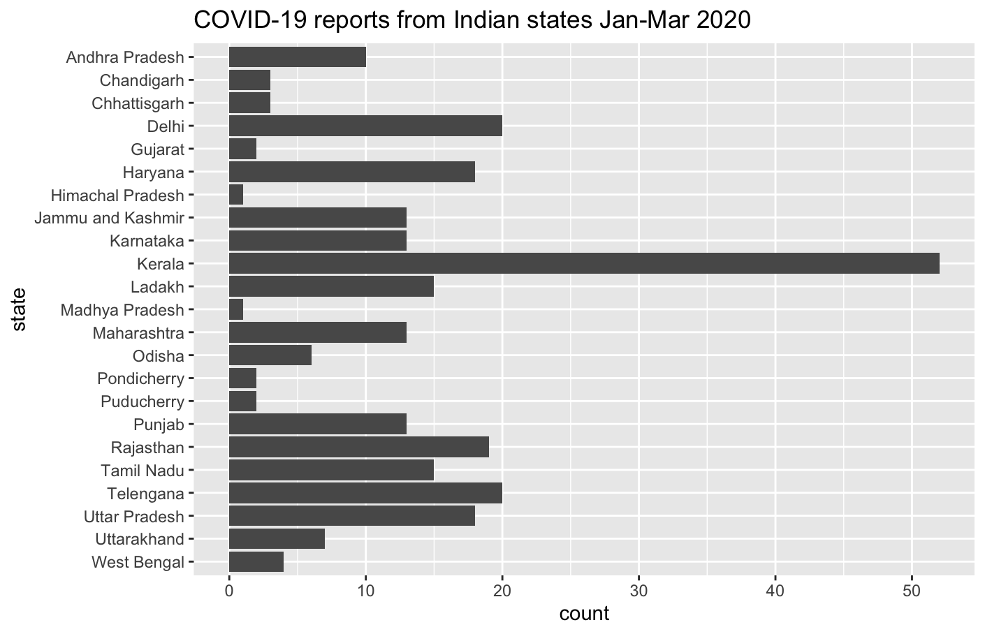
I made a bar chart showing the frequency of COVID-19 reports by state.

Covid19_India_Jan_20_Mar_20_ %>% 
  ggplot(aes(y = fct_rev(`State/UnionTerritory`))) + 
  geom_bar() + 
  labs(y = "state", title = "COVID-19 reports from Indian states Jan-Mar 2020")

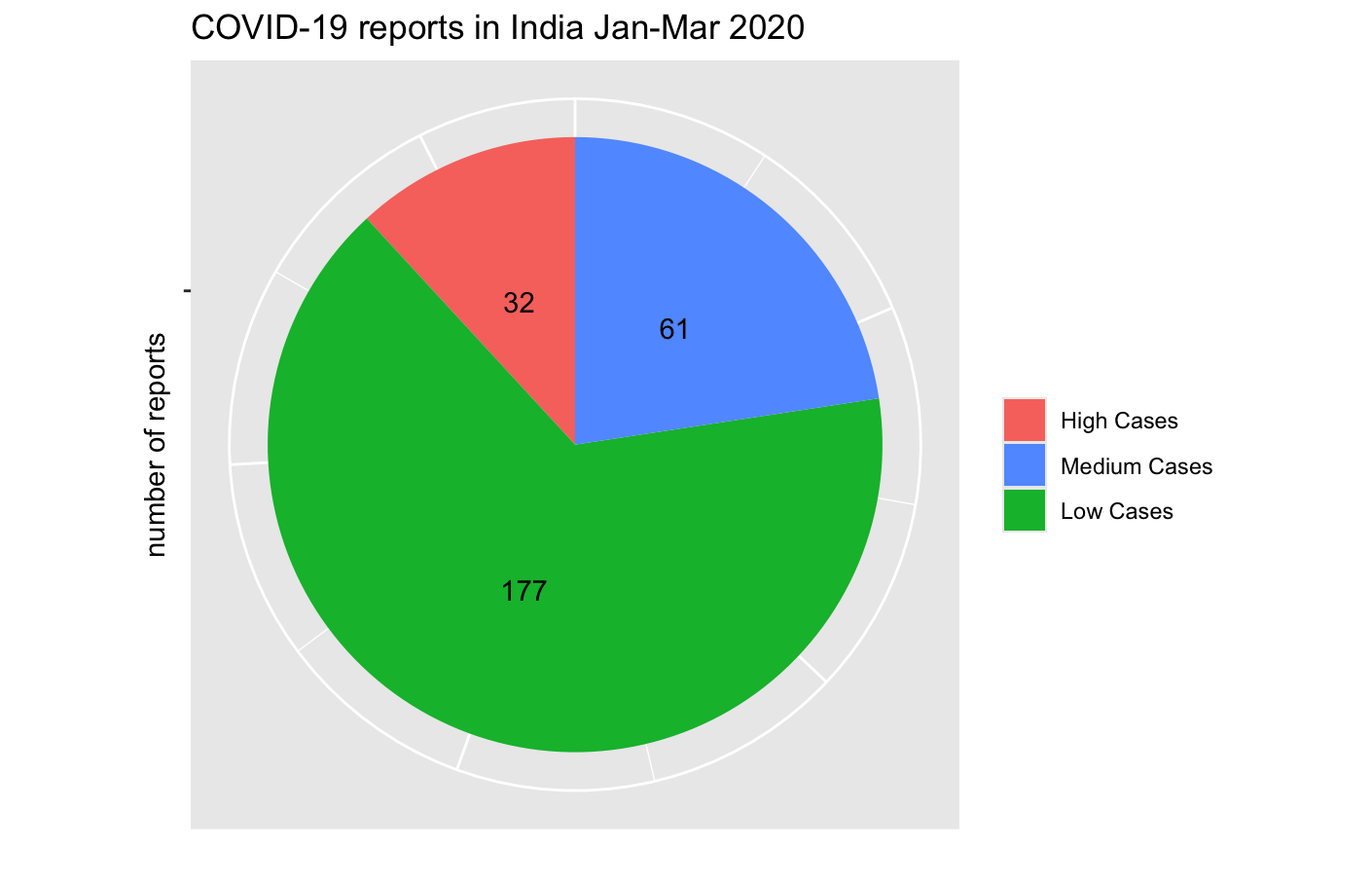
I made a pie chart showing the distribution of case severity levels, using total cases of Indian nationals and foreign nationals.

Covid19_India_Jan_20_Mar_20_ %>%
  group_by(case_level) %>% 
  summarise(count = n()) %>% 
  ggplot(aes(x = "", y = count, fill = case_level)) + 
  geom_col() + 
  coord_polar(theta = "y") + 
  geom_text(aes(label = count), position = position_stack(vjust = .5)) + 
  labs(x = "", y = "", fill = "", title = "COVID-19 reports in India Jan-Mar 2020") + 
  scale_fill_discrete(breaks = c("High Cases", "Medium Cases", "Low Cases")) + 
  theme(axis.text.x = element_blank())

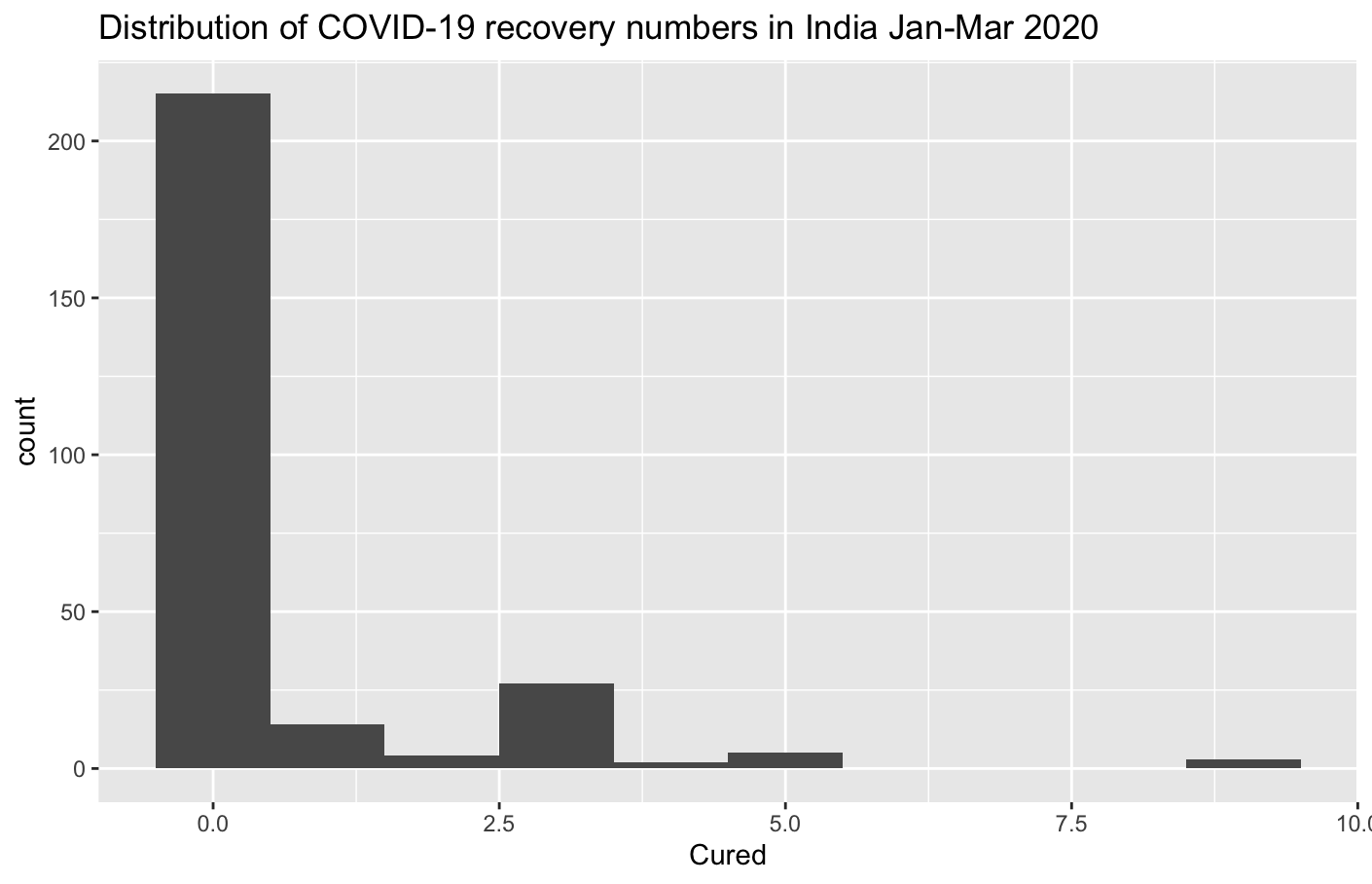
I made a histogram showing the distribution of recovery numbers.

Covid19_India_Jan_20_Mar_20_ %>% 
  ggplot(aes(Cured)) + 
  geom_histogram(bins = 10) + 
  labs(title = "Distribution of COVID-19 recovery numbers in India Jan-Mar 2020")

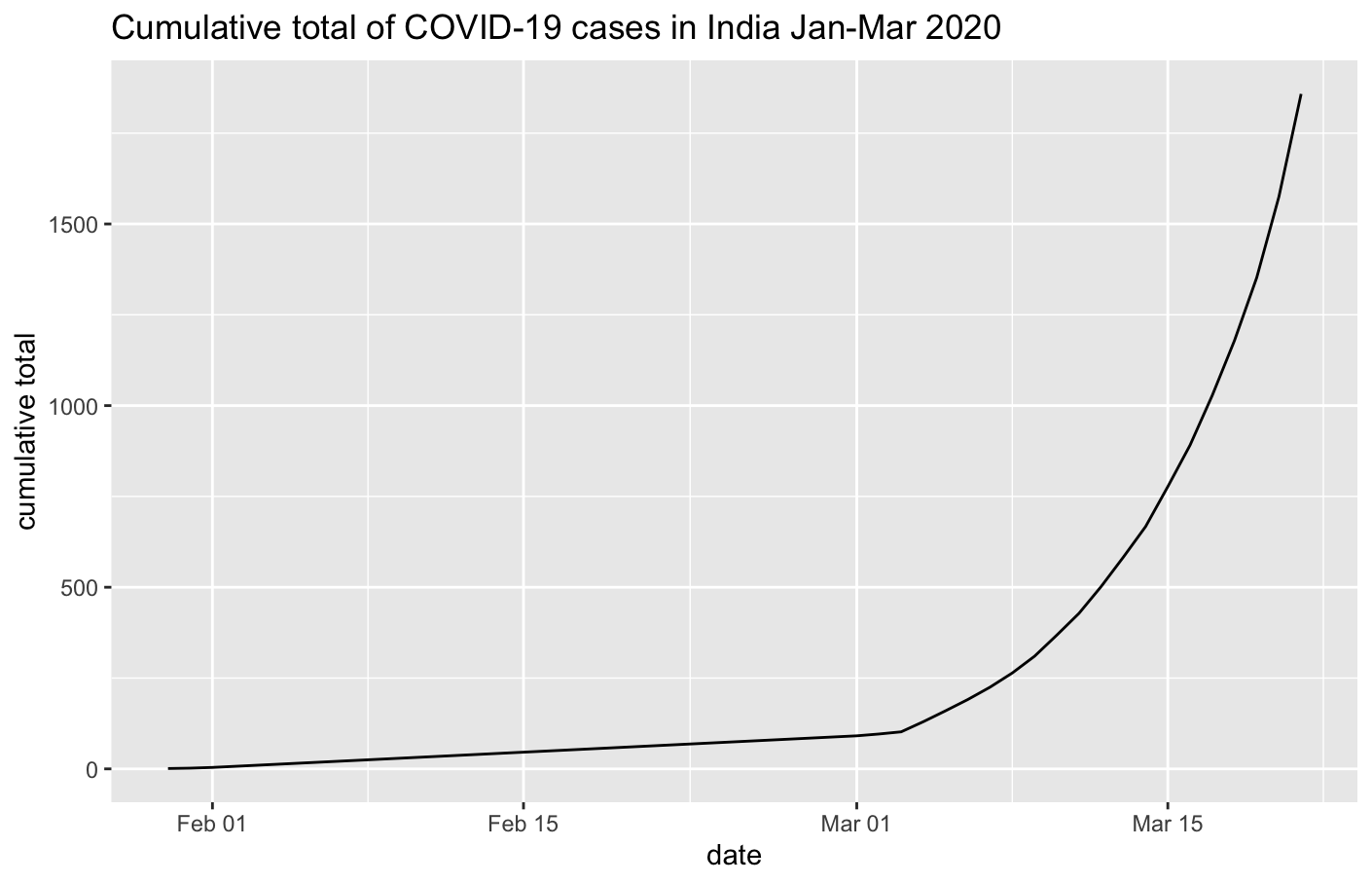
I made a line chart showing the trend of total cases over time.

Covid19_India_Jan_20_Mar_20_ %>% 
  arrange(date_converted) %>% 
  group_by(date_converted) %>% 
  summarise(total_cases = sum(ConfirmedIndianNational + ConfirmedForeignNational)) %>% 
  mutate(cum_sum = cumsum(total_cases)) %>% 
  ggplot(aes(date_converted, cum_sum)) + 
  geom_line() + 
  labs(title = "Cumulative total of COVID-19 cases in India Jan-Mar 2020", x = "date", y = "cumulative total")

I made a list of states showing total number of cases (Indian nationals and foreign nationals) in order from highest to lowest.

Covid19_India_Jan_20_Mar_20_ %>% 
  group_by(`State/UnionTerritory`) %>% 
  summarise(total_cases = sum(ConfirmedIndianNational + ConfirmedForeignNational)) %>% 
  arrange(desc(total_cases))

Here are the first ten results.

State/UnionTerritory	total_cases
Kerala	406
Maharashtra	355
Uttar Pradesh	214
Haryana	181
Rajasthan	175
Delhi	133
Karnataka	103
Telengana	74
Ladakh	71
Jammu and Kashmir	30

I made the same list again, but added the total number cured.

Covid19_India_Jan_20_Mar_20_ %>% 
  group_by(`State/UnionTerritory`) %>% 
  summarise(total_cases = sum(ConfirmedIndianNational + ConfirmedForeignNational), total_cured = sum(Cured)) %>% 
  arrange(desc(total_cases))

Here are the first ten results.

State/UnionTerritory	total_cases	total_cured
Kerala	406	57
Maharashtra	355	0
Uttar Pradesh	214	50
Haryana	181	0
Rajasthan	175	22
Delhi	133	22
Karnataka	103	2
Telengana	74	7
Ladakh	71	0
Jammu and Kashmir	30	0

We used the data to calculate probabilities using Bayes Theorem.

the probability that a randomly selected report comes from Kerala	$\mathrm{P(Kerala)}=\frac{\mathrm{52}}{\mathrm{270}}=\mathrm{19.3\%}$
the probability that a randomly selected report shows recoveries	$\mathrm{P(recoveries)}=\frac{\mathrm{55}}{\mathrm{270}}=\mathrm{20.4\%}$
the probability that a Kerala report shows recoveries	$\mathrm{P(recoveries|Kerala)}=\frac{\mathrm{19}}{\mathrm{52}}=\mathrm{36.5\%}$
the probability that a Delhi report shows recoveries	$\mathrm{P(recoveries|Delhi)}=\frac{8}{\mathrm{20}}=\mathrm{40\%}$
if a report shows recoveries, the probability that it came from Kerala	$\mathrm{P(Kerala|recoveries)}=\frac{\mathrm{P(recoveries|Kerala)}x\mathrm{P(Kerala)}}{\mathrm{P(recoveries)}}=\frac{\mathrm{0.365}x\mathrm{0.193}}{\mathrm{0.204}}=\mathrm{34.5\%}$

Working through these activities really helped me apply what I've learned about RStudio, and I'm sure I'll be using RStudio a lot in my career as a data scientist!