R for Data Science Exercises

Our task was to complete the exercises from chapters 5 and 7 of the brilliant R for Data Science textbook.

Chapter 5

These exercises were for practising handling data that is not "tidy" - data that doesn't follow these rules.

Each variable is a column; each column is a variable.
Each observation is a row; each row is an observation.
Each value is a cell; each cell is a single value.

Our task was to calculate tuberculosis rates from tables of "untidy" data, without making it tidy first.

table2 has a column for the value "cases" or "population" - this is "untidy" because these values could be column names.

table2 <- tribble(
  ~country, ~year, ~type, ~count,
  "Afghanistan", 1999, "cases", 745,
  "Afghanistan", 1999, "population", 19987071,
  "Afghanistan", 2000, "cases", 2666,
  "Afghanistan", 2000, "population", 20595360,
  "Brazil", 1999, "cases", 37737,
  "Brazil", 1999, "population", 172006362,
  "Brazil", 2000, "cases", 80488,
  "Brazil", 2000, "population", 174504898,
  "China", 1999, "cases", 212258,
  "China", 1999, "population", 1272915272,
  "China", 2000, "cases", 213766,
  "China", 2000, "population", 1280428583
)

First I extracted the values for "cases" and "population" into vectors.

table2_cases <- table2 |>
  filter(type == "cases") |>
  select(count) |>
  pull(count)

table2_population <- table2 |>
  filter(type == "population") |>
  select(count) |>
  pull(count)

I used these new vectors to create a vector for "rate" - the number of tuberculosis cases for every 10,000 people.

table2_rate <- table2_cases / table2_population * 10000

I looped backwards through table2 adding rows for "rate".

for(i in seq(nrow(table2), 1, by = -2)) {
  table2 <- add_row(table2, country = table2$country[i], year = table2$year[i], type = "rate", count = table2_rate[i/2], .after = i)
}

I used formatC to format the "count" column - format="f" removes scientific format, and drop0trailing = TRUE drops zeros after the decimal point.

table2$count <- formatC(table2$count, format= "f", drop0trailing = TRUE)

Here's the resulting table2.

	country	year	type	count
1	Afghanistan	1999	cases	745
2	Afghanistan	1999	population	19987071
3	Afghanistan	1999	rate	0.3727
4	Afghanistan	2000	cases	2666
5	Afghanistan	2000	population	20595360
6	Afghanistan	2000	rate	1.2945
7	Brazil	1999	cases	37737
8	Brazil	1999	population	172006362
9	Brazil	1999	rate	2.1939
10	Brazil	2000	cases	80488
11	Brazil	2000	population	174504898
12	Brazil	2000	rate	4.6124
13	China	1999	cases	212258
14	China	1999	population	1272915272
15	China	1999	rate	1.6675
16	China	2000	cases	213766
17	China	2000	population	1280428583
18	China	2000	rate	1.6695

table3 has a column for the values "cases" and "population" together - this is "untidy" because these values could be in separate columns.

table3 <- tribble(
  ~country, ~year, ~rate,
  "Afghanistan", 1999, "745/19987071",
  "Afghanistan", 2000, "2666/20595360",
  "Brazil", 1999, "37737/172006362",
  "Brazil", 2000, "80488/174504898",
  "China", 1999, "212258/1272915272",
  "China", 2000, "213766/1280428583"
)

I split the "rate" column into 2 values - cases and population.

cases_population <- str_split(table3$rate, "/")

I replaced the values in the "rate" column with new calculated values - the number of tuberculosis cases for every 10,000 people.

for(i in 1:nrow(table3)) {
  table3$rate[i] <- as.numeric(cases_population[[i]][1])/as.numeric(cases_population[[i]][2]) * 10000
}

Here's the resulting table3 - note that the rates are the same as in table2.

country	year	rate
Afghanistan	1999	0.372740958392553
Afghanistan	2000	1.29446632639585
Brazil	1999	2.19393047799011
Brazil	2000	4.61236337331918
China	1999	1.66749511667419
China	2000	1.6694878795907

Chapter 7

These exercises were for practising importing data with read_csv().

The first exercise has 5 read_csv() statements with errors. We had to work out the intention of each statement and correct it.

1. read_csv("a,b\n1,2,3\n4,5,6")

The intention is to read 3 columns and 2 rows, but column 3 doesn't have a name - I corrected it to this.

read_csv("a,b,c\n1,2,3\n4,5,6")

a	b	c
1	2	3
4	5	6

2. read_csv("a,b,c\n1,2\n1,2,3,4")

The rows have different numbers of columns - I corrected it to this.

read_csv("a,b,c,d\n1,2,3,4\n1,2,3,4")

a	b	c	d
1	2	3	4
1	2	3	4

3. read_csv("a,b\n\"1")

The quotes around the value are not closed, and the rows have different numbers of columns - I corrected it to this.

read_csv("a,b\n\"1\",\"2\"")

a	b
1	2

4. read_csv("a,b\n1,2\na,b")

The column names seem to be repeated - I corrected it to this.

read_csv("a,b\n1,2")

a	b
1	2

5. read_csv("a;b\n1;3")

The delimeter is a semicolon - I corrected it to this.

read_delim("a;b\n1;3", delim = ";")

a	b
1	3

The final exercise was practising referring to "nonsyntactic" column names - the column names are integers.

annoying <- tibble(
  `1` = 1:10,
  `2` = `1` * 2 + rnorm(length(`1`))
)

Extract the variable called "1".

annoying$`1`

 [1]  1  2  3  4  5  6  7  8  9 10

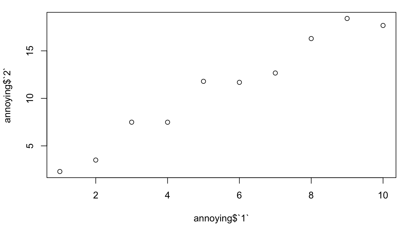
Plot a scatterplot of "1" versus "2".

plot(annoying$`1`, annoying$`2`)

Create a new column called "3", which is "2" divided by "1".

annoying$`3` <- annoying$`1` / annoying$`2`

annoying$`3`

 [1] 0.4346452 0.5703123 0.4004234 0.5342338 0.4240465 0.5135067 0.5526404 0.4910714
 [9] 0.4889729 0.5659152

Rename the columns to "one", "two" and "three".

annoying <- annoying %>% 
  rename(one = `1`, two = `2`, three = `3`)

	one	two	three
1	1	2.30072725631471	0.43464517458788
2	2	3.50685026436756	0.570312345617268
3	3	7.49206971481884	0.400423396230042
4	4	7.48735913301889	0.534233757047955
5	5	11.7911601781261	0.424046482658725
6	6	11.6843658769525	0.513506686044045
7	7	12.6664656044915	0.552640351189824
8	8	16.2909102699325	0.491071393031075
9	9	18.4059281805146	0.488972895674333
10	10	17.6704925840338	0.565915180487698

I thought these were excellent exercises, particularly the ones where we had to think about the intention of incorrect R code before correcting it.

I love using SQL, and R feels like the next logical step for me. These exercises really helped me look more deeply at the subtleties of R functions.